ANCHOR Visualization Tutorial

1. Access the ANCHOR homepage at http://structure.pitt.edu/anchor/

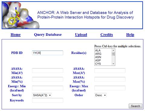
2. Click in Query Database.

3. On the query database form (below), type 1YCR on the PDB ID field and then click in Search to retrieve from the ANCHOR database the pre-computed data for the residues of the given PDB ID (p53-MDM2 protein-protein interaction).

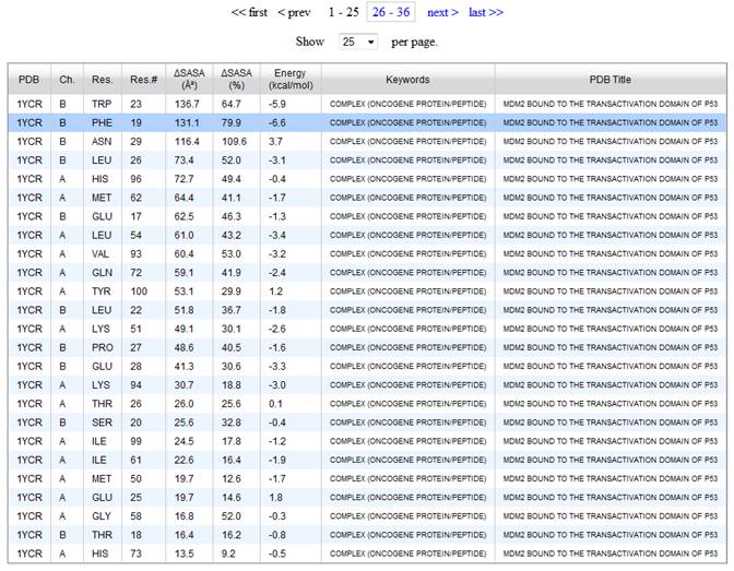
4. After a few seconds, a table with information about the residues is loaded at the bottom of the query form. By default, this list is sorted by decreasing order of the change in solvent accessible surface area upon binding (∆SASA). However, the user may change that behavior by setting the values of the fields Sort by and Order in the query form. Next, click for example on the second residue on the list, that is, B PHE 19.

5. Upon clicking on a residue from the hit list, a new window will pop up with the visualization tool (below). The visualization tool will automatically load the pdb file and show the selected residue as sticks. Protein chains nearby the selected residue chain are shown as a solvent accessible surface, color coded by atomic partial charges. On the right side of the window, there is a table showing information for the other residues in the same chain (chain B) as the selected residue (B PHE 19). On this table, click on the residues B TRP 23 and B LEU 23 and note that these residues now became visible. In order to zoom in around a residue, first click in Zoom In on the top-right side of the visualization window and then click on the residue on the table. Try to do that with residue B TRP 23.

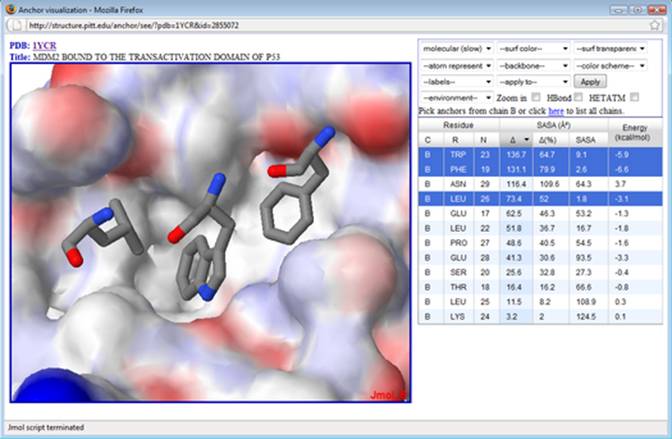
6. Next, select environment->’anchor+12A’ to show the residues surrounding the 3 selected residues. Select (a) ‘atom representation’->wireframe, (b) backbone->trace and (c) ‘apply to’->’anchor chain’ and then click on the button Apply. Next, select (a) ‘atom representation’->sticks and (b) ‘apply to’->’selected anchors’ and then click on the button Apply. At this point, you should be able to see the selected residues in sticks representation, the nearby residues in wireframe representation, and a backbone trace. Next, select surface->cavity. Then (a) ‘color scheme’->’receptor-anchor chains’ and button Apply. You should be able to end up similarly to the figure below.

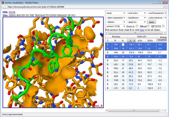
7. Finally, note that the selected anchor residues (in green sticks) from p53 bind to a large cavity (orange patch) in MDM2. These three residues are among those with the largest ∆SASA and lowest (i.e. favorable) predicted binding energy. Note that while ASN 29 has a large ∆SASA, it also has an unfavorable predicted energy (+3.7 kcal/mol), besides been located away from the other top ranked residues. Thus ASN 29 doesn’t seem to be a good anchor/hotspot for drug design. On the other hand, the three selected residues (PHE 19, TRP 23 and LEU 26) are indeed hotspots that have been exploited on the design of compounds that bind to MDM2 (see for example Doemling, A. (2008) Small molecular weight protein-protein interaction antagonists – an insurmountable challenge? Curr. Opin. Chem. Biol., 12(3), 281-291).